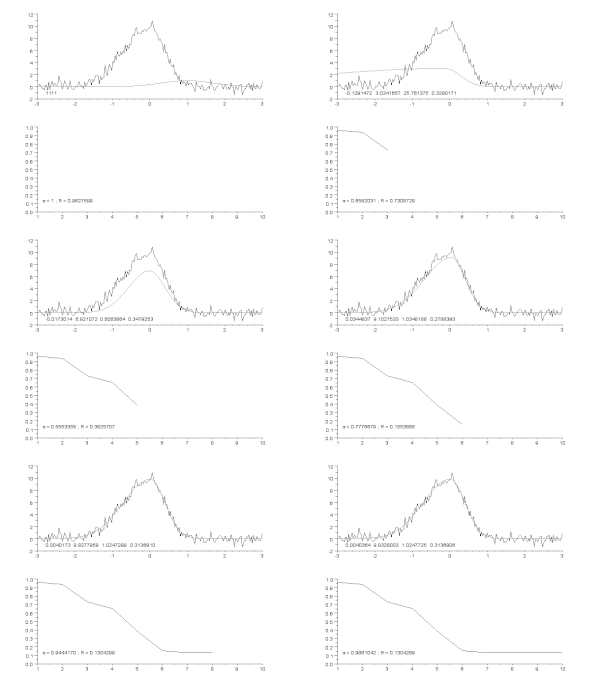
Gauss–Newton algorithm

Top: Raw data and model.
Bottom: Evolution of the normalised sum of the squares of the errors.
The Gauss–Newton algorithm is used to solve non-linear least squares problems, which is equivalent to minimizing a sum of squared function values. It is an extension of Newton's method for finding a minimum of a non-linear function. Since a sum of squares must be nonnegative, the algorithm can be viewed as using Newton's method to iteratively approximate zeroes of the components of the sum, and thus minimizing the sum. In this sense, the algorithm is also an effective method for solving overdetermined systems of equations. It has the advantage that second derivatives, which can be challenging to compute, are not required.
Non-linear least squares problems arise, for instance, in non-linear regression, where parameters in a model are sought such that the model is in good agreement with available observations.
The method is named after the mathematicians Carl Friedrich Gauss and Isaac Newton, and first appeared in Gauss' 1809 work Theoria motus corporum coelestium in sectionibus conicis solem ambientum.
Description
Given 


Starting with an initial guess 

where, if r and β are column vectors, the entries of the Jacobian matrix are

and the symbol 
At each iteration, the update 
With substitutions 


If m = n, the iteration simplifies to

which is a direct generalization of Newton's method in one dimension.
In data fitting, where the goal is to find the parameters 


Then, the Gauss–Newton method can be expressed in terms of the Jacobian 


Note that 


